by Sebastian Kohlstädt 1,2,Michael Vynnycky 1,3,* andStephan Goeke 41
Division of Processes, Department of Materials Science and Engineering, KTH Royal Institute of Technology, Brinellvägen 23, 100 44 Stockholm, Sweden
2Volkswagen AG—Division of Components Manufacturing, Dr. Rudolf-Leiding-Platz 1, 34225 Baunatal, Germany
3Department of Mathematics and Statistics, University of Limerick, Limerick V94 T9PX, Ireland
4Institute of Mechanics, Kassel University, Mönchebergstr. 7, 34125 Kassel, Germany*Author to whom correspondence should be addressed.
Abstract
This paper uses computational fluid dynamics (CFD), in the form of the OpenFOAM software package, to investigate the forces on the salt core in high-pressure die casting (HPDC) when being exposed to the impact of the inflowing melt in the die filling stage, with particular respect to the moment of first impact—commonly known as slamming. The melt-air system is modelled via an Eulerian volume-of-fluid approach, treating the air as a compressible perfect gas. The turbulence is treated via a Reynolds-averaged Navier Stokes (RANS) approach. The RNG k-ε and the Menter SST k-ω models are both evaluated, with the use of the latter ultimately being adopted for batch computations. A study of the effect of the Courant number, with a view to establishing mesh independence, indicates that meshes which are finer, and time steps that are smaller, than those previously employed for HPDC simulations are required to capture the effect of slamming on the core properly, with respect to existing analytical models and empirical measurements. As a second step, it is then discussed what response should be expected when this force, with its spike-like morphology and small force-time integral, impacts the core. It is found that the displacement of the core due to the spike in the force is so small that, even though the force is high in value, the bending stress inside the core remains below the critical limit for fracture. It can therefore be concluded that, when assuming homogeneous crack-free material conditions, the spike in the force is not failure-critical.Keywords: compressible two-phase flow; slamming; OpenFOAM; high-pressure die casting; lost salt cores; solid continuum mechanics
1. Introduction
High-pressure die casting (HPDC) is an important process for the manufacture of high-volume and low-cost automotive components, such as automatic transmission housings, crank cases and gear box components [1,2,3]. Liquid metal, generally aluminium or magnesium, is injected through a complex system of gates and runners and into the die at speeds of between 50 and 100 ms−1 at the ingate, and under pressures as high as 100 MPa [4].From an economic point of view, HPDC is typically constrained by a huge base investment in machinery and tooling, although this is alleviated by low incremental costs for each additional unit produced; in short, the process scales very well with increasing output. On the other hand, this complicates the task for the design engineer, who has to be sure about the viability of a process and manufactured parts before any budget is invested in tooling and machinery. One technological constraint to date is that there is no serial production, via HPDC, of parts with inlying hollow shapes or undercuts formed by lost cores, even though other casting techniques have employed lost cores for decades [1,4]. Nevertheless, several ideas for such products do already exist [5,6,7], and one material that has been put forward as a candidate for HPDC with lost cores is salt [6,8,9]. The basic idea of using salt cores is to block parts of the die volume by inserting cores as placeholders; in so doing, the melt will not penetrate into this space. The cores may then be removed after solidification and one creates undercuts or hollow sections with them, which may then later act as cooling or oil-flow channels [6,8,9].One way to determine whether lost cores are indeed a viable option for a given geometry is to employ numerical simulation—in particular, computational fluid dynamics (CFD) [10,11,12,13]. However, whereas the papers just mentioned focused on the flow of a melt past a core in more general terms, the particular focus of this paper shall be on determining the load on the solid core during the melt’s initial impact. This concept is often referred to as slamming, and is a phenomenon that is investigated more commonly in the context of naval architecture [14,15,16]; it occurs when a two-phase interface with one phase of high density—water—and another of lower density—air—hits an obstacle, for example, a ship. This can also be the case when investigating lost cores in high-pressure die casting, when the air surrounding the core is replaced by the much heavier melt. The particular scientific and technological issue of interest is the initial peak in the load that all previous simulations of high-pressure die casting and lost cores have predicted [10,11,12,13]; more precisely, we wish to investigate the core’s response to this load peak in more detail, in order to determine whether the core will fail as a result of it.
2. Model Equations and Simulation Methodology
2.1. Model Equations
As in our earlier CFD modelling of high-pressure die casting [12,17], we model the two-phase flow of molten metal and air by using the volume-of-fluid (VOF) method [18], wherein a transport equation for the VOF function, γ, of each phase is solved simultaneously with a single set of continuity and Navier-Stokes equations for the whole flow field; note also that γ, which is advected by the fluids, can thus be interpreted as the liquid fraction. Considering the molten melt and the air as Newtonian [19], compressible and immiscible fluids, the governing equations can be written as [20,21]
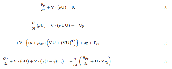
where t is the time, U the mean fluid velocity, p the pressure, g the gravity vector, Fs the volumetric representation of the surface tension force and T denotes the transpose. In particular, Fs is modelled as a volumetric force by the Continuum Surface Force (CSF) method [22]. It is only active in the interfacial region and formulated as Fs=σκ∇γ, where σ is the interfacial tension and κ=∇⋅(∇γ/|∇γ|) is the curvature of the interface; the significance of the term Ur in Equation (3) is explained shortly in Section 2.2. The material properties ρ and μ are the density and the dynamic viscosity, respectively, and are given by

where the subscripts g and l denote the gas and liquid phases, respectively. We take ρl,μg and μl to be constant, but assume the air to be an ideal gas, that is, its density changes with pressure and temperature; hence, the equation of state for our model reads
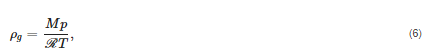
where M is the molecular weight for air, R is the universal gas constant and T is the temperature. This is a new unknown in the system and needs to be solved for via the heat equation [20,21],

where K=1/2U⋅U is the kinetic energy, cvg and cvl denote the specific heat capacities at constant volume for the gas and liquid phases, respectively, αeff is given by
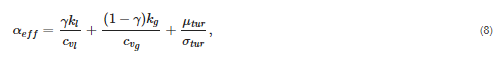
where kg and kl denote the thermal conductivities for the gas and liquid phases, respectively, and σtur is the turbulent Prandtl number, whose value is set to 0.9 [23]. Note that αeff resembles a phase-averaged thermal diffusivity that includes the contribution of turbulence, although it lacks a density term in the denominator. Furthermore, μtur in Equation (2) denotes the turbulent eddy viscosity, which will be calculated via the Menter SST k–ω model [24]; the equations for this model are summarized in the Appendix A.The major purpose of this paper is to calculate the forces on the core during slamming. Those are governed by the following formulae. For i=x,y, the total force acting on the core in direction i, Fi,tot, is given by

where Fi,p and Fi,s are pressure and viscous shear forces, respectively, and are given by
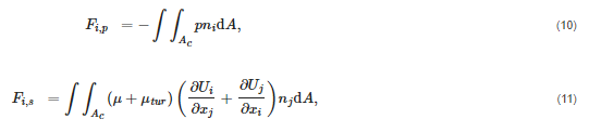
where U=(Ux,Uy) as the velocity and its components and Ac is the surface area of the core.The model two-dimensional (2D) geometry shown in Figure 1. This consists of two channel walls, an inlet, an outlet and a salt core that is located about the horizontal axis of symmetry of the channel. A summary of the mathematical expressions of the applied boundary conditions is presented in Table 1. In summary: the channel walls and the surface of the core are no-slip, zero heat-flux boundaries; the inlet velocity and temperature are prescribed; the outlet is at ambient pressure and heat conduction is negligible. In addition, there is always melt at the inlet, so that γ=1 there; at all other boundaries, γ satisfies a zero flux condition.

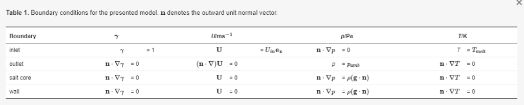
As for the initial conditions of the die, the cavity is filled with air (γ = 0) that is at rest (U = 0), at ambient temperature (T = Tamb) and at atmospheric pressure (p = pamb). The initial conditions for the turbulence model are set via the length scale of the largest eddies and the turbulence intensity. Those quantities were set to 2 mm and 5 %, respectively.What is now still missing are the material properties of the phases. Those are presented in Table 2. Note that we have taken ρl and μl to be constant, even though they would in general depend on the temperature. The reason for taking them to be constant is that the temperature of the melt will not change appreciably from Tmelt during the filling, in view of the zero heat flux boundary conditions that are being applied; on the other hand, ρg may change appreciably, as the gas will heat up from its initial ambient temperature and experience a significant increase in pressure, both of which are accounted for via Equation (6). One additional comment concerns the specific heat capacities cpg and cpl: the index p means that their values have been measured and documented for constant pressure, which are more commonly tabulated rather than cvg or cvl. Equation (7), however, requires cv. This conversion can be conducted via the value of the isentropic expansion factor or heat capacity factor, which can for air be assumed to be constant and equal to cpg/cvg = 1.4 in the given temperature range [12,25,26]. For the aluminum melt, this additional step is not necessary, as it was treated as being incompressible; thus, cvl = cpl.Table 2. Model parameters. The parameters for gas are those for air; those for metal are for the alloy AlSi9Cu3 [12,19,27].
Table 2. Model parameters. The parameters for gas are those for air; those for metal are for the alloy AlSi9Cu3 [12,19,27].
| cvg | 720 J kg−1 K−1 |
|---|---|
| cvl | 1000 J kg−1 K−1 |
| kg | 0.026 W m−1K−1 |
| kl | 70 W m−1K−1 |
| M | 0.028 kg mol−1 |
| Tamb | 293 K |
| pamb | 105 Pa |
| Tmelt | 823 K |
| Uin | 10, 20 m s−1 |
| μg | 1.8×10⁻⁵ Pa s |
| μl | 1.62×10⁻³ Pa s |
| ρl | 2520 kg m−3 |
| σ | 0.629 N m−1 |
2.2. Simulation Methodology
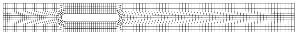
To solve the above equations, the OpenFOAM software package [28,29,30,31] was used, due to the niche nature of the field of application, as well as to make use of its extendability. OpenFOAM has most of its applications designed for solving fluid mechanics problems [29,32] and applies the finite volume method [23,33,34] to solve them. With the later aim of scaling the model to complex industrial 3D-geometries in mind, OpenFOAM is also a very powerful tool, since the distribution of a case to a huge number of CPU-cores is not limited due to license restrictions, as is the case with commercial CFD codes. In particular, we used the compressibleInterFoam solver, which handles two compressible, non-isothermal immiscible fluids using a VOF interface-capturing approach. The solver also uses the multi-dimensional universal limiter with explicit solution (MULES) scheme for interface compression, which introduces a supplementary velocity field, Ur, in the vicinity of the interface, as seen in Equation (3); in doing so, the local flow steepens the gradient and the interface becomes sharper and more pristine. A typical form for Ur is Ur=min(U,max(U)), as given by Reference [20]. Further benefits that accrue from using OpenFOAM for this application that its implementation of the Menter SST k-ω model has previously been shown to be robust, and to give results that are in excellent agreement with experimental data [35,36]. Moreover, by use of a function object called forces that is already pre-implemented in OpenFOAM, the forces required in Equations (10) and (11) can be readily calculated.The corresponding mesh for the 2D-geometry shown in Figure 1 is illustrated in Figure 2. This is a structured mesh consisting of one layer of hexahedral cells. It is also parameterized and can therefore easily be refined for later mesh independence studies. For this purpose, the OpenFOAM utility refineMesh was used that, by default, halves the mesh spacing upon execution, that is, quadrupling the cell count for a 2D mesh as in Figure 2. This simplified model was used for efficiency reasons in order to establish that the newly installed tool yields sensible results.
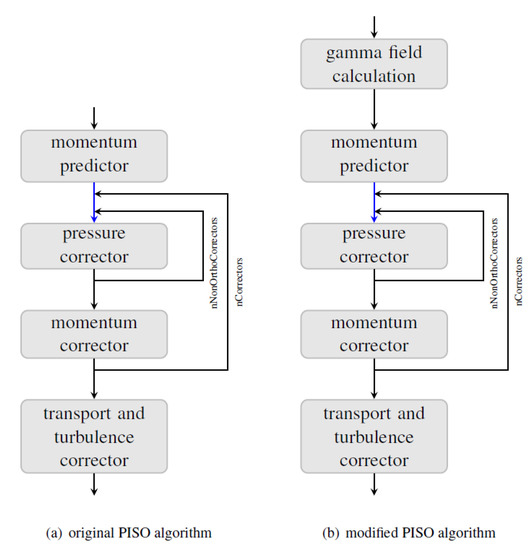
Lastly, as this is a rather complex flow problem in the context of CFD research, it is worthwhile to look at the solution algorithm a little more closely. In order to do that, Figure 3 is presented. Here, the standard PIMPLE algorithm, a combination of PISO (Pressure Implicit with Splitting of Operator) [37] and SIMPLE (Semi-Implicit Method for Pressure-Linked Equations) [38], was modified and, for this purpose, an additional step was added that solved the transport equation of the phase variable γ according to Equation (3) at the beginning of the solution algorithm, that is, before the momentum predictor. Figure 3 shows the original PISO algorithm on the left and on the right the reader sees the implemented extension of it including the additional step for the phase field for handling the two-phase flow. The corrector loops can either be broken by a residual or a maximum number criterion. One additional comment for the sake of completeness is that the outermost loop for the increasing time step is omitted, as the chart only shows the processes that occur within each time step.
3. Results and Discussion
In this section, we present the results of the numerical simulations. The principal aim of these is to determine the magnitudes of the forces which act on the salt core, with a view to being able to infer whether an actual salt core would be able to withstand such forces in practice. As one of the diagnostics of the computations, we consider first the slamming factor, so as to link our results to analytical expressions for this quantity that are available in the field of marine technology.
3.1. The Concept of the Dimensionless Slamming Factor
Following the results of recently published articles on salt cores in high-pressure die casting [10,12,13,17], in almost every simulation where the core was treated as rigid, the signature peak mentioned in Section 1 appeared in a plot of the force exerted on the core as a function of time. The ambition here was therefore to investigate its nature in more detail. This will be done by introducing the dimensionless slamming factor, Cs, which is defined asCs=FρRU2l,(12)where F is the force, and is given byF=F2x,tot+F2y,tot−−−−−−−−−−√,(13)with Fx,tot and Fy,tot being computed according to Equations (9)–(11); Cs also depends on the density, ρ, the undisturbed melt velocity U, the radius of the core, R, and its length, l. Analytical progress was made by von Karman [39] and Wagner [40] to determine this slamming factor in the context of marine technology, with the result that according to von Karman the slamming factor for a cylinder was π, while Wagner put it at 2π. More recent studies [14,41], however, indicate that the value according to von Karman represents a lower limit of the slamming factor, while the Wagner model acts as an upper cap. Both models also fail to provide an evolution of the value over time. Campbell and Weynberg [15,42] present a model that offers results based on empirical data to determine the plot over time, according to the formulaCs=F(t)ρRU2l=5.151+9.5UtR−1+0.275UtR−1.(14)The letters in Equation (14) represent the same quantities as in Equation (12).The introduced dimensionless slamming factor makes the calculated results independent of the ingate velocity or geometric dimensions. This is further illustrated in the following plot. Figure 4 shows that the calculated slamming factor is the same no matter whether it is being evaluated for an ingate velocity of 10 or 20 ms−1. Those values for Uin were used for U for calculating the slamming factor according to Equations (12)–(14).
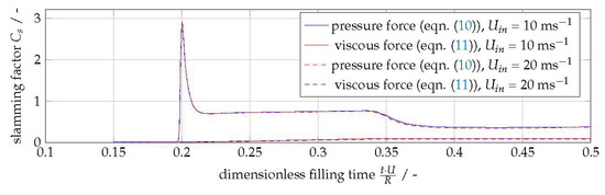
Figure 4. Normalized forces on the core for a mesh resolution of 0.3 mm.
3.2. Determining the Slamming Factor with Respect to Mesh Resolution
The model setup was calibrated with existing data on similar cases, such as the water entry of an axisymmetric projectile [43] with similar Reynolds numbers and also for the feature of the pile-up effect [41,44,45], wherein a jet is formed near the intersection with the initial water surface.Applying the model to the previously introduced case, Figure 5, Figure 6 and Figure 7 show the temporal development of the phase distribution, the pressure and the velocity at impact on the core. Please note that, although the model is non-isothermal, it does not take the temperature difference between the core, the walls and the melt into account, in the sense that zero heat-flux boundary conditions are applied at all solid boundaries (see Table 1). The actual fluid flow and heat transfer in the near-wall area may therefore differ in reality due to heat transfer-induced effects.
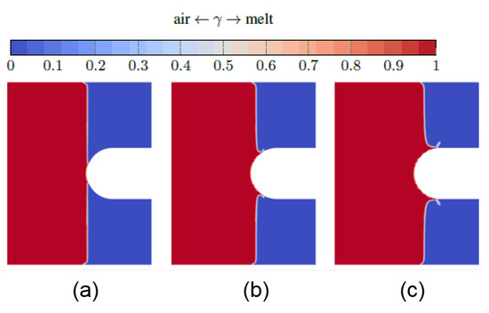
Figure 5. Phase distribution of the melt at impact and immediately afterwards: (a) t⋅UR = 0.2; (b) t⋅UR = 0.205; (c) t⋅UR = 0.21. Here, U=Uin with Uin = 20 ms−1.
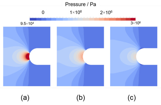
Figure 6. The pressure field at the times of impact and immediately afterwards: (a) t⋅UR = 0.2; (b) t⋅UR = 0.205; (c) t⋅UR = 0.21. Here, U=Uin with Uin = 20 ms−1.
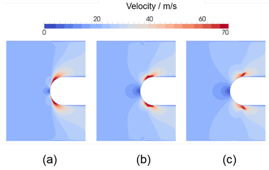
Figure 7. The velocity magnitude field at the times of impact and immediately afterwards: (a) t⋅UR = 0.2; (b) t⋅UR = 0.205; (c) t⋅UR = 0.21. Here, U=Uin with Uin = 20 ms−1.After calibrating the setup, it was time to proceed to evaluating the forces on the core and to benchmark them with previously published data. The first thing to determine was the necessary mesh resolution in order to compute plausible results for the slamming factor. The results of this mesh resolution study are presented in Figure 8. A meticulous investigation of this phenomenon of slamming showed that, with generally used meshing standards in industry-oriented computations and mesh spacings in the range of 1 mm [10], the CFD simulation underpredicts the value of the slamming factor (see Figure 8). It becomes evident that the simulation requires a mesh as fine as a spacing of 0.3 mm in order for the computed result for Cs to be above the lower limit of the slamming factor according to the von Karman model. This is significantly lower than the typical mesh spacing that was used in Reference [10] and requires a mesh for this rather small geometry to consist in total of 60,000 cells, albeit being a 2D mesh. Transferring these results onto a real-world casting geometry that includes salt cores and designing a 3D mesh according to these findings would, in turn, produce a mesh that it would be completely impractical to use with currently available computational capacity.
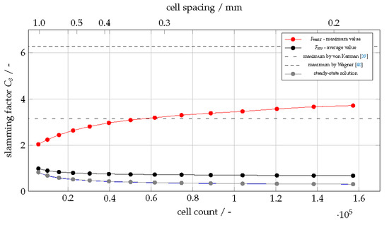
Figure 8. Mesh study of the slamming factor in comparison with the models by von Karman [39] and Wagner [40]. Here, Uin = 20 ms−1.While Figure 8 showed that coarser meshes underpredict the peak in the force, the stationary value of the force tends to be overpredicted the coarser the mesh is. From a design engineer’s point of view, this is a beneficial outcome as it includes a built-in safety factor into the design of a devised product. Note also that the stationary or steady-state solution in Figure 8 refers to the constant value for Cs that is obtained once the melt front is well past the salt core; see, for example, Figure 4.Figure 9 shows this study’s result in comparison with the findings of previously published articles [15,39,40,46,47]. The results are plotted for a mesh spacing of 0.025 mm. Technically, only a refinement of the cells in the near core area would be necessary. However, given the fact that then the structured nature and the numerical benefits that come along with it would have to be sacrificed, this opportunity was forgone here as the domain was sufficiently small and calculation efficiency was not a benchmark in this academic study. It should be noted that the analytical models start with t = 0 at the point of impact, whereas for our numerical simulation t=0 denotes the time a which melt start to enter the cavity; for this reason, the simulation time values were therefore adjusted so that t=0 in Figure 9 corresponds to the time when melt first hits the core, with the consequence that negative values of t appear in this figure.
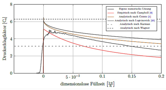
Figure 9. Comparison of the computed result with reference studies in previously published articles; mesh cell spacing 0.025 mm.Figure 9 shows also the values for several other models, among them the static von Karman [39] and Wagner [40] models, as well as more recent models that also represent the development of the force over time [46,47]. It can be concluded that this study’s assessment of the slamming factor agrees very well with earlier authors’ findings. One interesting observation of the result from the present volume-of-fluid model is that its increase is, compared to the mostly analytical models, more gradual. The other models feature a sharp step-like increase in value, resembling the morphology of a Heaviside function [48].The reason for this gradual increase is to be found most likely inside the volume-of-fluid approach itself. As Equations (4) and (5) illustrated, the material properties are being averaged by their volume fraction, γ. Another reason for this feature is to be found in the numerical approach of this study, where the numerics are known to smear out the interface of volume-of-fluid simulations [49] and therefore artificial interface compression terms are to be introduced into the partial differential equation for the volume fraction [12,49], Equation (3). This effect of a non-discrete interface causes additional problems in stability of the interFoam solver-family in the sense of spurious parasitic velocities at the interface, and several strategies to mitigate the effects towards a sharper interface have since been proposed [50,51,52,53]. We can conclude that, taking into account Figure 8 and Figure 9, one has, for the given boundary conditions, to maintain at least a mesh fineness corresponding to a spacing of 0.2 mm, in order to reach a value for Cs above the limit defined by von Karman in Reference [39], if one wants to achieve a proper result for the slamming factor. Transferring this finding to more applicable designs in industry, it underscores the need for mesh refinement near a salt core boundary if the load is to be evaluated correctly.
3.3. Effect of Turbulence
The aspect of turbulence treatment on the slamming factor in the simulations was also evaluated during the investigations. Figure 10 features this result. Two different turbulence models were benchmarked against each other for the given case and the different mesh spacings, as illustrated in Figure 10. The benchmarked turbulence models are Menter’s SST k-ω model [24,54] and the RNG k-ε model [55]. The reason why those two were picked is that the Menter model was proven to be of excellent stability and accuracy proven in studies published by other authors [35] and our own results published in previous papers [11,12]. The RNG-model was selected as it is the standard of the commercial CFD casting software Flow-3D Cast. Both turbulence models belong to the RANS-model family (Reynolds-Averaged-Navier-Stokes equations).
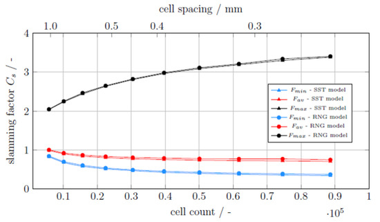
Figure 10. Influence of the selected turbulence model on the computed result for the slamming factor.As is evident from Figure 10, the selection of the turbulence model is of minor importance. Even with different mesh spacings, the result of the slamming factor stayed more or less the same. This is plausible, as the main contribution to the slamming results from the pressure forces on the core—an effect documented in more detail in Reference [12]. For those forces, the momentum of the melt is more important compared to other factors in the fluid. This is also easy to comprehend with the introduced formulae in Equations (10) and (11). One sees here that the only quantity that is influenced by the turbulence model is μtur, while all the others do not directly depend on it. This turbulent eddy viscosity, however, only appears in the formula for the viscous forces, which are of negligible importance as seen in Figure 4.
3.4. Effect of Courant Number
One might now argue that the presented strong mesh dependency of the results is the consequence of the simulation time-step size being Courant number-controlled [56], and hence that an automatic reduction of the mesh spacing should lead to a shorter time step, Δt, in consequence. In order to eliminate this possibility, studies with different Courant numbers were also conducted; in particular, each cell’s local Courant number is calculated, and the solver then sets a value for Δt so that these local Courant numbers are not greater than some maximum allowable value that is specified by the user. The result of this investigation is shown in Figure 11. In Figure 11a, the values for Fstat are shown, whereas Figure 11b shows the values for Fmax. Fstat calculates the slamming factor value via the average force computed while the denser phase surrounds the cores, while Fmax uses the peak force value. Although the latter in particular oscillates somewhat, there is no obviously visible trend that would support the hypothesis that only reducing Δt would also lead to a more physical value for the slamming factor on a coarser mesh. The values for Fstat and Fmax are the same for a Courant number range from 0.1 to 2, while at the same time the difference caused by the different mesh resolution was clearly visible. In conclusion, a mesh spacing of 0.6 mm with a Courant number of 2 leads to values much closer to reality for the peak in the force than a mesh resolution of 1 mm with a maximum Courant number of 0.1. But, even for a mesh resolution of 0.6 mm, the computed values for the peak in the force are significantly below the lower bound given by the von Karman model (π).
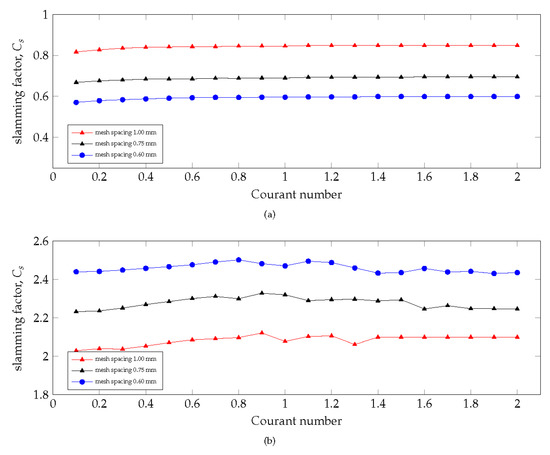
Figure 11. Results of the time step size Δt study: (a) Results for Fstat; (b) Results for Fmax.
3.5. Response of the Core to the Spike-Like Force Impact
Although it is academically interesting to determine the value for the slamming factor as precisely as possible, the general underlying question is also whether such a small force-time interval is failure-critical for salt cores in high-pressure die casting in general. We will therefore in the following present a couple of considerations to assess the necessity for the engineer to keep the slamming factor below a certain level.If one, for this purpose, leaves the field of 2D considerations and imagines how a beam of length 70 mm that is situated within the die facing the inflowing melt stream orthogonally would react to the inflowing melt and the slamming, one would make the following observations. The consideration is of course based on the assumption that the inflowing melt stream stays as thin as in the test case, a fact that has emerged in more application-oriented studies [12,17]. In general, any force impacting on the core at one point cannot travel through the solid body faster than the speed of sound,vs=Kρs−−−√,(15)with vs being the speed of sound in salt, K being the bulk modulus for salt cores and ρs being the density of salt cores. K is related to the documented quantities for salt cores [17] via References [57,58]K=E3(1−2ν),(16)with E as the Young’s modulus and ν as the Poisson ratio. Assuming ρs as 2056 kg m−3, ν as 0.21 and E as 1.5×10¹⁰ Pa [17], Equations (15) and (16) yield the speed of sound in salt as 2048 ms−1. Based on Figure 4, one can now assume 0.02 s as a scale for the dimensionless filling time, yielding 3.5×10⁻⁶ s as an absolute time scale during which the peak force acts on the core. Together with the calculated speed of sound, this means that a stress signal travelling a distance below 10 mm through the core, that is, referring back to the beam with 70 mm in length, would not even be able to reach the bearing.If we further assume a slamming factor of 32π, as reported in Figure 9, the absolute force according to Equation (12) is slightly below 1400 N. Now, applying Newton’s second law,F=ma,(17)where F is the force, m is the mass and a is the acceleration, integrating (17) twice with respect to t, and assuming the initial velocity to be zero and a to be constant, to obtains=12at2,(18)where s denotes distance, one may get an idea of how far the centre of the core travels. Based on the calculations above for the distance travelled in two directions of the beam and the reported dimensions of the core in Figure 1, neglecting the round edges, one obtains a displaced mass of 0.02 kg leading, with the previously calculated value for the force, to an acceleration of 6.6×10⁻⁶ ms−2 and in turn to a displacement of the core section of 4×10⁻⁷ m in the direction of the mean flow, according to Equation (18). Three-point bending tests with salt cores, conducted by the authors [17], show that the tested specimens manufactured via pressing and sintering [59] are, even at room temperature, capable of undergoing displacements of this scale without cracking, provided that they are free of internal cracks, that is, meaning that the continuum mechanics approach can be applied.In turn, this leads to the conclusion that, due to the short time scales of the slamming effects, they are not to be considered failure-critical for the salt core. Based on the presented knowledge, only a small segment of the core will be displaced by the spike in the force, causing the core in turn to vibrate. The time scale of the impact will be too small to reach the core bearings and produce a counterforce. Due to the displacement, the core will start to vibrate before being permanently deformed by the steady-state force. Since this steady-state force will be present for a longer period of time, this may in the end be failure-critical. To finally conclude the discussion, the reader should bear two additional things in mind. The results presented, although relying heavily on dimensionless numbers, are hugely geometry-, parameter- and, most notably, ingate/impact velocity-dependent. One must therefore be careful to transfer these findings to other geometries and setups; on the other hand, it is highly recommended to apply the presented CFD approach to the geometry at hand. Secondly, the assumption of the core being crack-free may also be flawed with respect to reality. It may therefore be possible that salt cores, as the material salt is of a ceramic nature, will most often contain small cracks. It thus provides scope for future research work to develop a model for assessing how long potential cracks are allowed to be in order to withstand the slamming impact. Another interesting direction will be to measure not only the displacement of a die casting, as was done in Reference [17], but also the forces on it.As a practical conclusion, this also suggests that pre-heated cores that are warmer than room temperature may yield a higher fraction of castings with intact cores and thus yield channel geometries within the tolerance limit. Higher temperatures naturally make it more likely that the material will fail in a ductile way, rather than in a brittle way.
4. Conclusions
In the course of this paper, the presented research work showed that the slamming phenomenon is something that is in general underestimated by state-of-the-art CFD simulations in industry that have used typical mesh spacings of 1 mm. We have found that the mesh resolution has to be increased by a factor of 40 in order for the computed slamming factor to be in the range of existing analytical results of empirical measurements. Interestingly, the reduction of the time step size, Δt, did not show any impact on the proper estimation of the slamming factor’s value. The contribution of the turbulence in this study was found to be negligible and the mathematical justification for this was shown with the presented formulae; this echoes the findings and conclusions of more application-related studies [12]. It remains a topic for scientific debate as regards what response of the core the slamming peak in the force actually causes inside the material. This paper provides a reasoning based on simple continuum mechanics formulae that the core will, for the given parameters, be only slightly displaced and thus in turn only vibrate—thus rendering the slamming impact to be a non-failure-critical phenomenon. The reader is reminded that the provided results are only valid for the presented boundary conditions and transferring them to other setups has to be handled with care. It is never possible, without the detailed geometric constraints and boundary conditions, to decide whether a salt core solution for high-pressure die casting will be viable. Future research will be undertaken to measure the force inside a die during filling and also to combine the concept of slamming with the laws of fracture mechanics.
Author Contributions
Conceptualization, S.K.; methodology, S.K.; software, S.K. and S.G.; validation, S.K.; formal analysis, S.K., M.V.; investigation, all; writing–original draft preparation, S.K. and M.V.; writing–review and editing, S.K. and M.V.; supervision, M.V.; project administration, S.K. and M.V.; funding acquisition, S.K. All authors have read and agreed to the published version of the manuscript.
Funding
This research received no external funding.
Informed Consent Statement
Not applicable.
Data Availability Statement
The data presented in this study are available on request from the first author.
Conflicts of Interest
The authors declare no conflict of interest. The funders had no role in the design of the study; in the collection, analyses, or interpretation of data; in the writing of the manuscript, or in the decision to publish the results.
Appendix A. The Menter SST k-ω Model (Menter 1994)
The equations for the Menter Shear Stress Transport (SST) k-ω turbulence model, where k is the turbulence kinetic energy and ω is the specific rate of dissipation of the turbulence kinetic energy, areD(ρk)Dt=τ:∇U−β∗ρωk+∇⋅[(μ+σkμtur)∇k],(A1)D(ρω)Dt=ρΓμturτ:∇U−βρω2+∇⋅[(μ+σωμtur)∇ω]+2(1−F1)ρσω2ω∇k⋅∇ω,(A2)whereDDt=∂∂t+U⋅∇,and withτ=μtur(∇U+(∇U)T−23(∇⋅U)δ)−23ρkδ,(A3)where δ is the Kronecker delta and β∗=0.09. The model constants σk,σω,β and Γ are given byφ=F1φ1+(1−F1)φ2for φ=(σk,σω,β,Γ), withσk1=0.85,σω1=0.5,β1=0.0750,σk2=1.0,σω2=0.856,β2=0.0828,Γi=βi/β∗−σωiκ2/β∗−−√,i=1,2,where κ=0.41. In addition,F1=tanh(arg41),(A4)witharg1=min[max(k−−√0.09ωy,500μy2ρω),4ρσω2kCDkωy2],(A5)where y is the distance to the nearest surface and CDkω is the positive portion of the cross-diffusion term in Equation (10), that is,CDkω=max(2ρσω2ω∇k⋅∇ω,10−20),(A6)and the turbulent viscosity, μtur, is given byμtur=a1ρkmax(a1ω,ΩF2),(A7)where Ω is the absolute value of the vorticity, that is, Ω=|∇×U|, and F2 is given byF2=tanh(arg22),(A8)wherearg2=max(2k−−√0.09ωy,500μy2ρω),(A9)and a1=0.31.
References
- Kaufmann, H.; Uggowitzer, P. Metallurgy and Processing of High-Integrity Light Metal Pressure Castings; Schiele & Schön: Berlin, Germany, 2007. [Google Scholar]
- Nogowizin, B. Theorie und Praxis des Druckgusses, 1st ed.; Schiele & Schoen: Berlin, Germany, 2010. [Google Scholar]
- Brunnhuber, E. Praxis der Druckgussfertigung; Schiele & Schoen: Berlin, Germany, 1991. [Google Scholar]
- Campbell, J. Complete Casting Handbook: Metal Casting Processes, Metallurgy, Techniques and Design; Elsevier Science: Amsterdam, The Netherlands, 2015. [Google Scholar]
- Jelínek, P.; Adámková, E. Lost cores for high-pressure die casting. Arch. Foundry Eng. 2014, 14, 101–104. [Google Scholar] [CrossRef]
- Kohlstädt, S.; Rabus, U.; Goeke, S.; Kuckenburg, S. Verfahren zur Herstellung Eines Metallischen Druckgussbauteils Unter Verwendung Eines Salzkerns Mit Integrierter Stützstruktur und Hiermit Hergestelltes Druckgussbauteil. DE Patent DE10,201,410,221,359A1, 21 April 2016. [Google Scholar]
- Schneider, T.; Kohlstädt, S.; Rabus, U. Gehäuse mit Druckgussbauteil zur Anordnung Eines Elektrischen Fahrmotors in Einem Kraftfahrzeug und Verfahren zur Herstellung eines Druckgussbauteils. DE Patent DE10,201,410,221,358A1, 21 April 2016. [Google Scholar]
- Graf, E.; Soell, G. Vorrichtung zur Herstellung Eines Druckgussbauteils mit Einem Kern und Einem Einlegeteil. DE Patent DE10,145,876A1, 10 April 2003. [Google Scholar]
- Graf, E.; Söll, G. Verfahren zur Herstellung Eines Zylinderkurbelgehäuses. WO Patent WO2,008,138,508A1, 20 November 2008. [Google Scholar]
- Fuchs, B.; Körner, C. Mesh resolution consideration for the viability prediction of lost salt cores in the high pressure die casting process. Prog. Comput. Fluid Dyn. 2014, 14, 24–30. [Google Scholar] [CrossRef]
- Kohlstädt, S.; Vynnycky, M.; Gebauer-Teichmann, A. Experimental and numerical CHT-investigations of cooling structures formed by lost cores in cast housings for optimal heat transfer. Heat Mass Trans. 2018, 54, 3445–3459. [Google Scholar] [CrossRef]
- Kohlstädt, S.; Vynnycky, M.; Neubauer, A.; Gebauer-Teichmann, A. Comparative RANS turbulence modelling of lost salt core viability in high pressure die casting. Prog. Comput. Fluid Dyn. 2019, 19, 316–327. [Google Scholar] [CrossRef]
- Fuchs, B.; Eibisch, H.; Körner, C. Core viability simulation for salt core technology in high-pressure die casting. Int. J. Met. 2013, 7, 39–45. [Google Scholar] [CrossRef]
- Fuchs, V. Numerische Modellierung von Fluid-Struktur-Wechselwirkungen an Wellenbeaufschlagten Strukturen; Kassel University Press GmbH: Kassel, Germany, 2014. [Google Scholar]
- Campbell, T.; Weynberg, P. Measurement of Parameters Affecting Slamming—Final Report; Technical Report, Wolfson Marine Craft Unit Report No. 440; University of Southampton: Southampton, UK, 1980. [Google Scholar]
- Abrate, S. Hull slamming. Appl. Mech. Rev. 2011, 64, 060803. [Google Scholar] [CrossRef]
- Kohlstädt, S.; Vynnycky, M.; Jäckel, J. Towards the modelling of fluid-structure interactive lost core deformation in high-pressure die casting. Appl. Math. Mod. 2020, 20, 319–333. [Google Scholar] [CrossRef]
- Hirt, C.; Nichols, B. Volume of fluid (VOF) method for the dynamics of free boundaries. J. Comput. Phys. 1981, 39, 201–225. [Google Scholar] [CrossRef]
- Dahle, A.; Arnberg, L. The rheological properties of solidifying aluminum foundry alloys. JOM 1996, 48, 34–37. [Google Scholar] [CrossRef]
- Ferrer, P.; Causon, D.; Qian, L.; Mingham, C.; Ma, Z. A multi-region coupling scheme for compressible and incompressible flow solvers for two-phase flow in a numerical wave tank. Comput. Fluids 2016, 125, 116–129. [Google Scholar] [CrossRef]
- Mayon, R.; Sabeur, Z.; Tan, M.Y.; Djidjeli, K. Free surface flow and wave impact at complex solid structures. In Proceedings of the 12th International Conference on Hydrodynamics, Egmond aan Zee, NL, USA, 18–23 September 2016. [Google Scholar]
- Brackbill, J.; Kothe, D.; Zemach, C. A continuum method for modeling surface tension. J. Comput. Phys. 1992, 100, 335–354. [Google Scholar] [CrossRef]
- Versteeg, H.; Malalasekera, W. An Introduction to Computational Fluid Dynamics: The Finite Volume Method; Pearson Education Limited: London, UK, 2007. [Google Scholar]
- Menter, F. 2-equation eddy-viscosity turbulence models for engineering applications. AIAA J. 1994, 32, 1598–1605. [Google Scholar] [CrossRef]
- Koch, M.; Lechner, C.; Reuter, F.; Köhler, K.; Mettin, R.; Lauterborn, W. Numerical modeling of laser generated cavitation bubbles with the finite volume and volume of fluid method, using OpenFOAM. Comput. Fluids 2016, 126, 71–90. [Google Scholar] [CrossRef]
- White, F. Fluid Mechanics, 7th ed.; McGraw-Hill: New York, NY, USA, 2011. [Google Scholar]
- Assael, M.; Kakosimos, K.; Banish, R.; Brillo, J.; Egry, I.; Brooks, R.; Quested, P.; Mills, K.; Nagashima, A.; Sato, Y.; et al. Reference data for the density and viscosity of liquid aluminum and liquid iron. J. Phys. Chem. Ref. Data 2006, 35, 285–300. [Google Scholar] [CrossRef]
- Jasak, H.; Jemcov, A.; Tukovic, Z. OpenFOAM: A C++ Library for Complex Physics Simulations. In Proceedings of the International Workshop on Coupled Methods in Numerical Dynamics IUC, Dubrovnik, Croatia, 19–21 September 2007. [Google Scholar]
- Jasak, H. OpenFOAM: Open source CFD in research and industry. Int. J. Naval Archit. Ocean Eng. 2009, 1, 89–94. [Google Scholar]
- Weller, H.; Tabor, G.; Jasak, H.; Fureby, C. A tensorial approach to computational continuum mechanics using object orientated techniques. Comput. Phys. 1998, 12, 620–631. [Google Scholar] [CrossRef]
- Maric, T.; Höpken, J.; Mooney, K. Openfoam Technology Primer; Stan Mott: Hannover, Germany, 2014. [Google Scholar]
- Chen, G.; Xiong, Q.; Morris, P.; Paterson, E.; Sergeev, A.; Wang, Y. OpenFOAM for computational fluid dynamics. Not. AMS 2014, 61, 354–363. [Google Scholar] [CrossRef]
- Jasak, H. Error Analysis and Estimation for the Finite Volume Method with Applications to Fluid Flows. Ph.D. Thesis, Imperial College London (University of London), London, UK, 1996. [Google Scholar]
- Droniou, J. Finite volume schemes for diffusion equations: Introduction to and review of modern methods. Math. Model. Methods Appl. Sci. 2014, 24, 1575–1619. [Google Scholar] [CrossRef]
- Robertson, E.; Choudhury, V.; Bhushan, S.; Walters, D. Validation of OpenFOAM numerical methods and turbulence models for incompressible bluff body flows. Comput. Fluids 2015, 123, 122–145. [Google Scholar] [CrossRef]
- Higuera, P.; Lara, J.; Losada, I. Simulating coastal engineering processes with OpenFOAM®. Coast. Eng. 2013, 71, 119–134. [Google Scholar] [CrossRef]
- Issa, R. Solution of the implicitly discretised fluid flow equations by operator-splitting. J. Comput. Phys. 1986, 62, 40–65. [Google Scholar] [CrossRef]
- Patankar, S.; Spalding, D. A calculation procedure for heat, mass and momentum transfer in three-dimensional parabolic flows. In Numerical Prediction of Flow, Heat Transfer, Turbulence and Combustion; Elsevier: Berlin/Heidelberg, Germany, 1983; pp. 54–73. [Google Scholar]
- von Karman, T.H. The Impact on Seaplane Floats during Landing; Technical Report; National Advisory Committee on Aeronautics: Washington, DC, USA, 1929; p. 8. [Google Scholar]
- Wagner, H. Über Stoß- und Gleitvorgänge an der Oberfläche von Flüssigkeiten. Zamm J. Appl. Math. Mech. Angew. Math. Und Mech. 1932, 12, 193–215. [Google Scholar] [CrossRef]
- Wienke, J. Druckschlagbelastung auf schlanke zylindrische Bauwerke durch brechende Wellen: Theoretische und großmaßstäbliche Laboruntersuchungen. Ph.D. Thesis, TU Braunschweig, Braunschweig, Germany, 2001. [Google Scholar]
- Campbell, T.; Weynberg, P. An Investigation into Wave Slamming Loads on Cylinders; Technical Report, Wolfson Marine Craft Unit Report No. 317; University of Southampton: Southampton, UK, 1977. [Google Scholar]
- Bodily, K.; Carlson, S.; Truscott, T. The water entry of slender axisymmetric bodies. Phys. Fluids 2014, 26, 072108. [Google Scholar] [CrossRef]
- Wienke, J.; Sparboom, U.; Oumeraci, H. Breaking wave impact on a slender cylinder. In Coastal Engineering 2000; ASCE: Reston, VA, USA, 2001; pp. 1787–1798. [Google Scholar]
- Ghadimi, P.; Dashtimanesh, A.; Djeddi, S.R. Study of water entry of circular cylinder by using analytical and numerical solutions. J. Braz. Soc. Mech. Sci. Eng. 2012, 34, 225–232. [Google Scholar] [CrossRef]
- Cointe, R.; Armand, J.L. Hydrodynamic impact analysis of a cylinder. J. Offshore Mech. Arct. Eng. 1987, 109, 237–243. [Google Scholar] [CrossRef]
- Logvinovich, G. Hydrodynamics of Free-Boundary Flows; Israel Program for Scientific Translation: Jerusalem, Israel, 1972. [Google Scholar]
- Duff, G.; Naylor, D. Differential Equations of Applied Mathematics; Wiley: New York, NY, USA, 1966. [Google Scholar]
- Rusche, H. Computational Fluid Dynamics of Dispersed Two-Phase Flows at High Phase Fractions. Ph.D. Thesis, Imperial College London (University of London), London, UK, 2003. [Google Scholar]
- Bo, W.; Grove, J.W. A volume of fluid method based ghost fluid method for compressible multi-fluid flows. Comput. Fluids 2014, 90, 113–122. [Google Scholar] [CrossRef]
- Fedkiw, R.; Aslam, T.; Merriman, B.; Osher, S. A non-oscillatory Eulerian approach to interfaces in multimaterial flows (the ghost fluid method). J. Comput. Phys. 1999, 152, 457–492. [Google Scholar] [CrossRef]
- Roenby, J.; Bredmose, H.; Jasak, H. A computational method for sharp interface advection. R. Soc. Open Sci. 2016, 3, 160405. [Google Scholar] [CrossRef]
- Vukčević, V. Numerical Modelling of Coupled Potential and Viscous Flow for Marine Applications. Ph.D. Thesis, Fakultet strojarstva i brodogradnje, Sveučilište u Zagrebu, Zagreb, Croatia, 2016. [Google Scholar]
- Menter, F.; Kuntz, M.; Langtry, R. Ten years of industrial experience with the SST turbulence model. Turbul. Heat Mass Transf. 2003, 4, 625–632. [Google Scholar]
- Yakhot, V.; Orszag, S.A.; Thangam, S.; Gatski, T.B.; Speziale, C.G. Development of turbulence models for shear flows by a double expansion technique. Phys. Fluids A Fluid Dyn. 1992, 4, 1510–1520. [Google Scholar] [CrossRef]
- Courant, R.; Friedrichs, K.; Lewy, H. On the partial difference equations of mathematical physics. IBM J. Res. Dev. 1967, 11(2), 215–234. [Google Scholar] [CrossRef]
- Beitz, W.; Shields, M.; Dubbel, H.; Davies, B.; Küttner, K. DUBBEL—Handbook of Mechanical Engineering; Springer: London, UK, 2013. [Google Scholar]
- Salencon, J.; Lyle, S. Handbook of Continuum Mechanics: General Concepts—Thermoelasticity; Physics and Astronomy Online Library; Springer: Berlin, Germany, 2001. [Google Scholar]
- Groezinger, D. Water-Soluble Salt Cores. U.S. Patent US8,403,028B2, 26 March 2013. [Google Scholar]